4 Congestion

Congestion occurs when available least-cost energy cannot be delivered to some loads because transmission facilities do not have sufficient capacity to deliver the energy. When the least-cost, available energy cannot be delivered to load in a transmission-constrained area, higher cost units in the constrained area must be dispatched to meet that load. The result is the price of energy in the constrained area will be higher than in the unconstrained area because of the combination of transmission limitations and the costs of local generation.

Congestion Rents on Interties

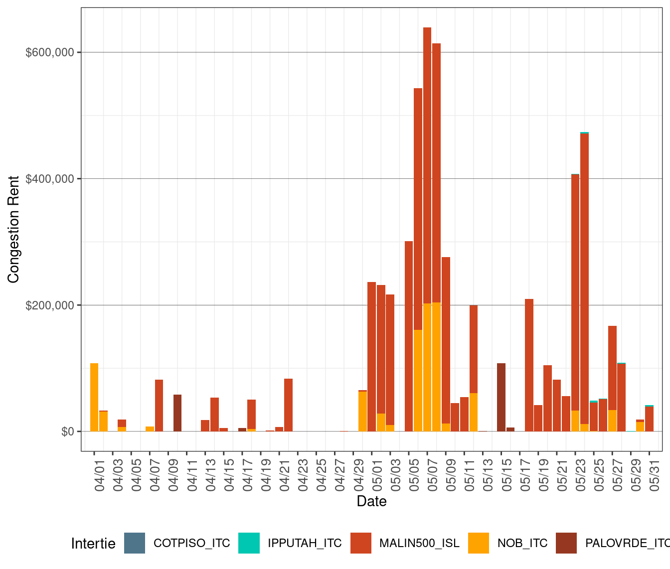
Figure 7 below illustrates the IFM congestion costs on interties. The congestion cost is calculated as shadow price ($/MWh) of the intertie constraint multiplied by the flow (MW) on the intertie. The cumulative total congestion rent for interties in May rose to $5.29 million from $0.60 million in April. Majority of the congestion rents in this month accrued on Malin500 (83 percent) and NOB (15 percent) intertie. The congestion rent on Malin500 increased to $4.38 million in May from $0.31 million in April. Malin was derated throughout this month due to various outages including the outages of Malin-Round Mountain #2 line, Table Mountain 500 kV breaker, and Table Mountain-Tesla 500 kV line. The congestion rent on NOB went up to $0.77 million in May from $0.22 million in April.

Figure 7: IFM (Day-Ahead) Congestion Rents by Intertie

Congestion Rents on Transmision Lines and Transformers

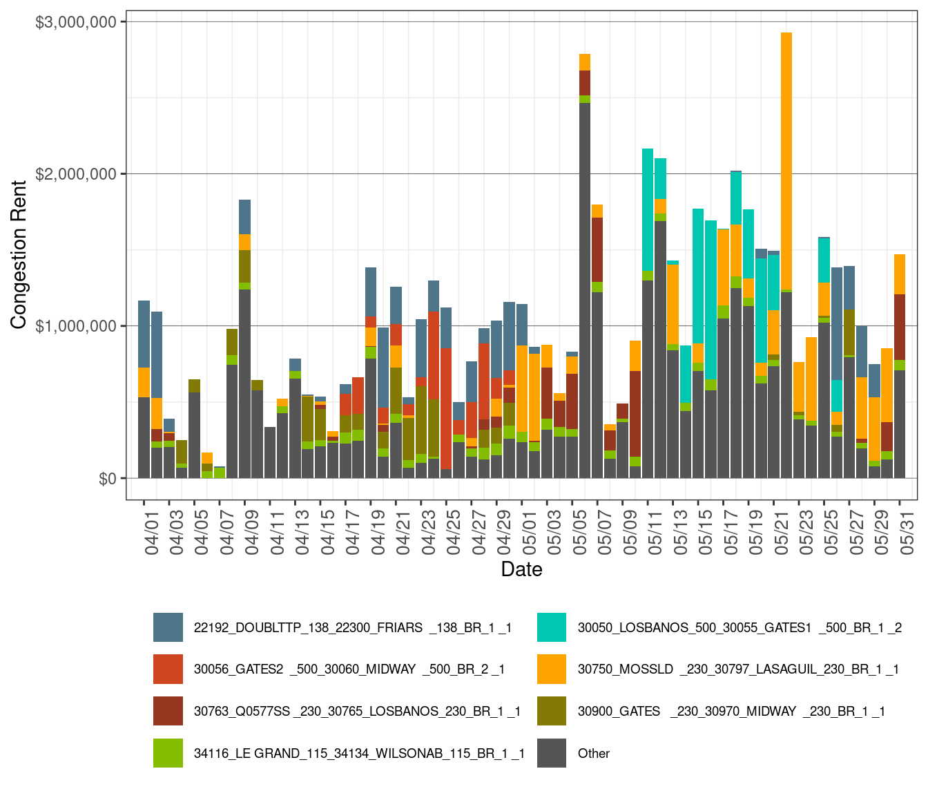
Figure 8 illustrates IFM congestion rents by transmission lines and transformers. The congestion cost is calculated as the shadow price ($/MWh) of the constraint multiplied by the flow limit (MW).

Figure 8: IFM (Day-Ahead) Congestion Rents by Transmission Lines and Transformers

Congestion Rents on Nomograms

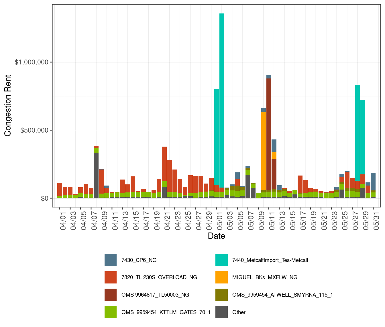
Figure 9 illustrates IFM congestion rents by nomogram. The congestion rent is calculated as the shadow price ($/MWh) of the constraint multiplied by the flow limit (MW).

Figure 9: IFM (Day-Ahead) Daily Congestion Rents by Nomogram

Congestion Rents on Nodal Group Constraints

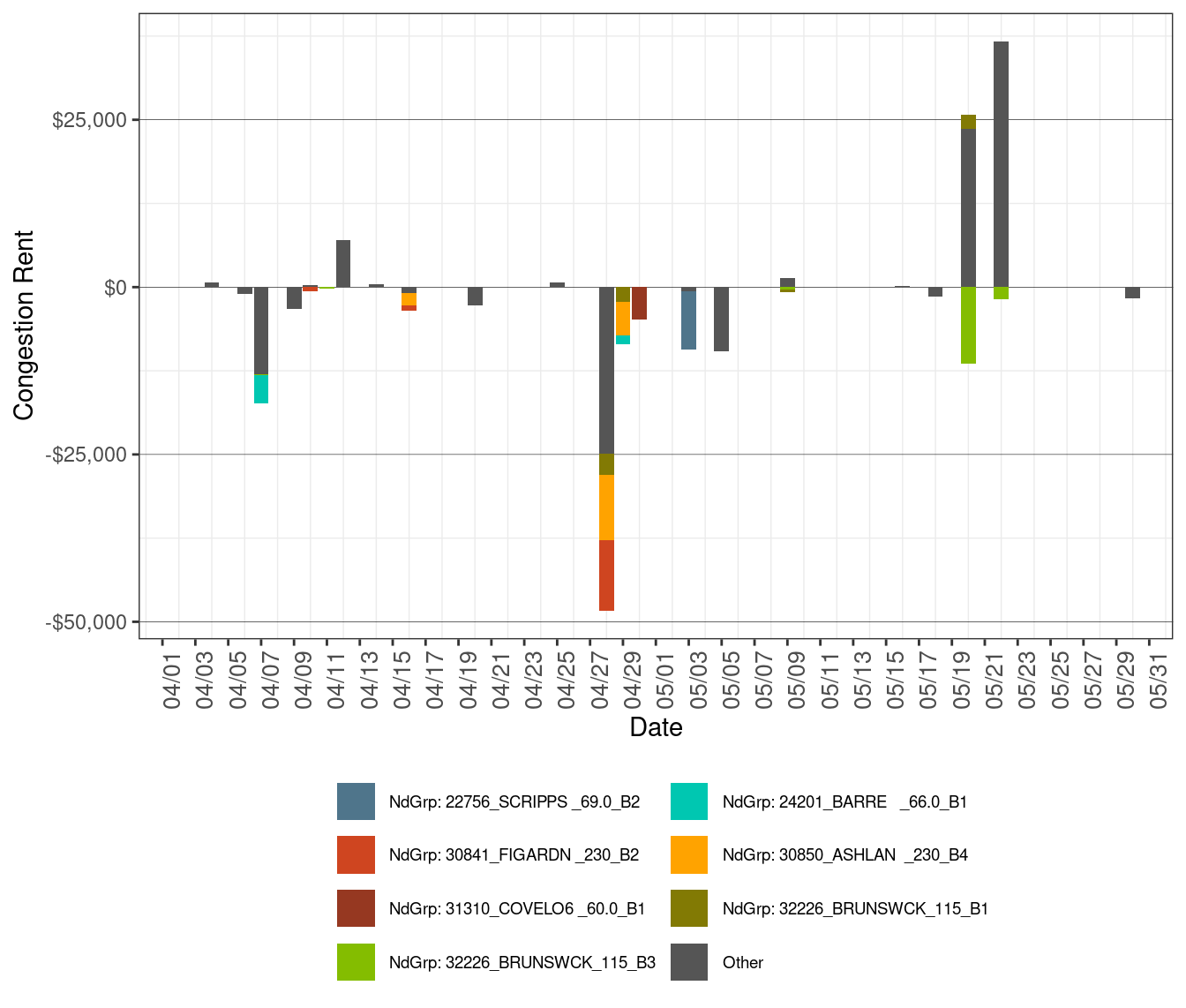
Figure 10 illustrates IFM congestion rents by nodal group constraints. The congestion rent is calculated as the shadow price ($/MWh) of the constraint multiplied by the flow limit (MW).

Figure 10: IFM (Day-Ahead) Daily Congestion Rents by Nodal Group Constraints