Section 4 Congestion

Congestion occurs when available least-cost energy cannot be delivered to some loads because transmission facilities do not have sufficient capacity to deliver the energy. When the least-cost, available energy cannot be delivered to load in a transmission-constrained area, higher cost units in the constrained area must be dispatched to meet that load. The result is the price of energy in the constrained area will be higher than in the unconstrained area because of the combination of transmission limitations and higher cost local generation. In other words, load in the constrained area will pay a higher price for power delivered over the transmission line than the price paid to generation for the power supplied to that transmission line. The difference between the amount paid by load and exports and the amount paid to generation and imports is the congestion rent. Congestion rent is usually returned back to transmission ratepayers (consumers) given that they have paid the costs of transmission infrastructure through network charges, specifically, the Transmission Access Charge (TAC).

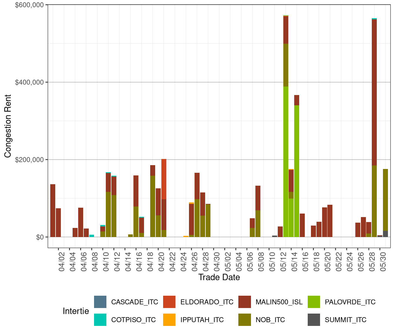
Congestion Rents on Interties

Figure 4.1 below illustrates the IFM congestion rents on interties. The hourly congestion rent is calculated as the shadow price ($/MWh) of the intertie constraint multiplied by the flow limit (MW) on the intertie constraint. The daily congestion rent is the sum of the hourly congestion rents collected on the intertie constraint for all hours of the trading day.

The cumulative total congestion rent for interties increased to $2.49 million in May from $1.89 million in the previous month. Majority of the congestion rents in May accrued on MALIN500_ISL(42.5%), NOB_ITC(23%) and PALOVRDE_ITC(33.3%). The congestion rent on MALIN500_ISL inter-tie in May increased to $1,058,121 from $947,693 in the previous month, while corresponding value of PALOVRDE_ITC in May increased to $827,875 from $0 in the April.

Figure 4.1: IFM (Day-Ahead) Congestion Rents by Intertie

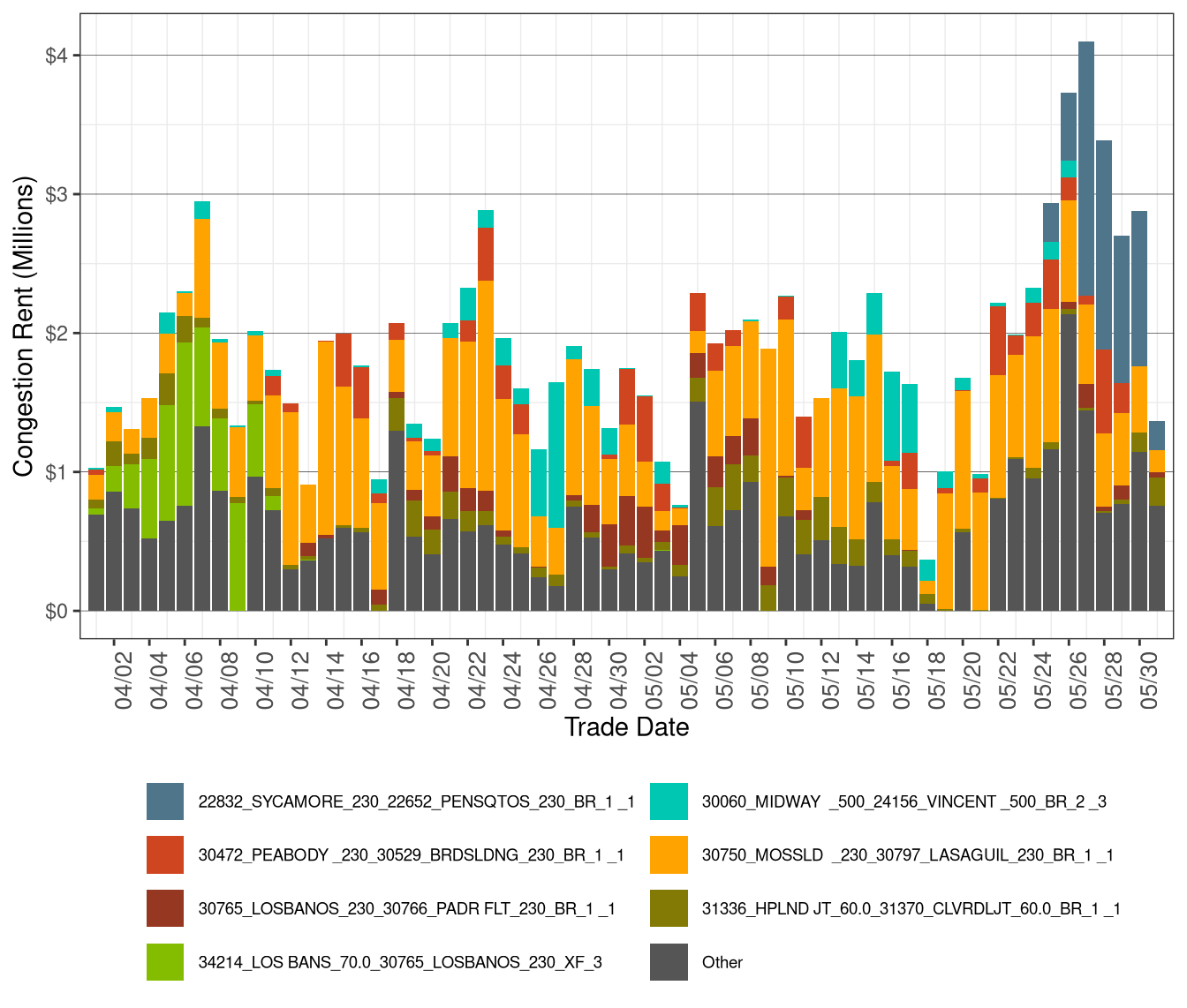
Congestion Rents on Transmission Lines and Transformers

Figure 4.2 illustrates IFM congestion rents by transmission lines and transformers. The hourly congestion rent is calculated as the shadow price ($/MWh) of the constraint multiplied by the flow limit (MW). The daily congestion rent is the sum of the hourly congestion rents collected on the transmission constraint for all hours of the trading day.

Figure 4.2: IFM (Day-Ahead) Congestion Rents by Transmission Lines and Transformers

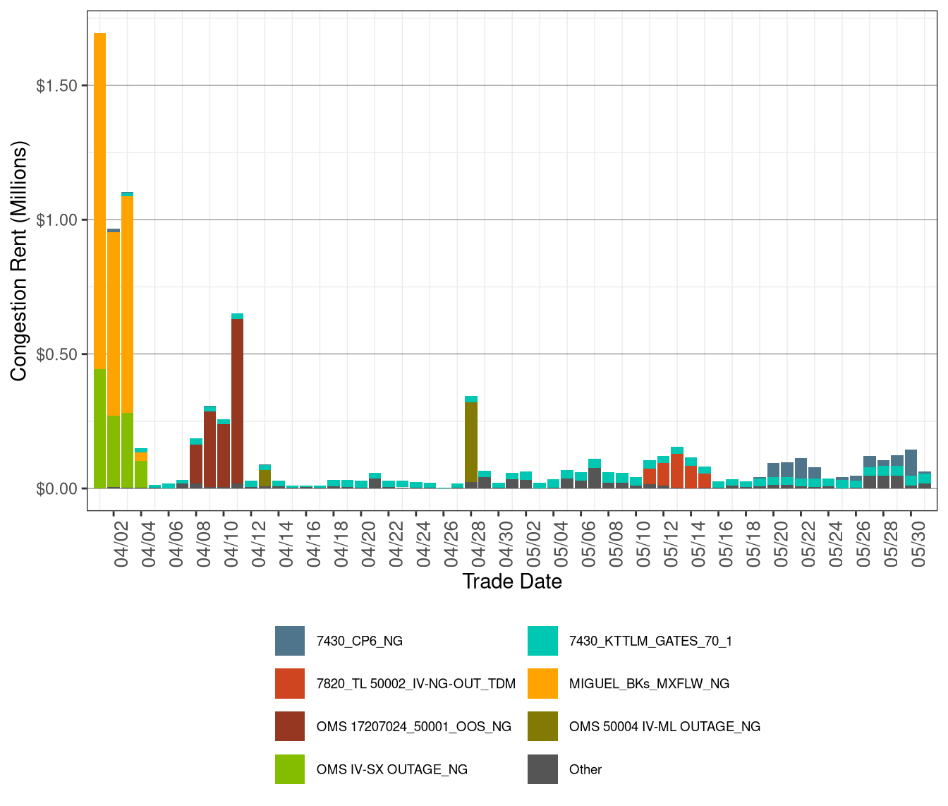
Congestion Rents on Nomograms

Figure 4.3 illustrates IFM congestion rents by nomogram. The hourly congestion rent is calculated as the shadow price ($/MWh) of the nomogram constraint multiplied by the flow limit (MW). The daily congestion rent is the sum of the hourly congestion rents collected on the nomogram constraint for all hours of the trading day.

Figure 4.3: IFM (Day-Ahead) Daily Congestion Rents by Nomogram

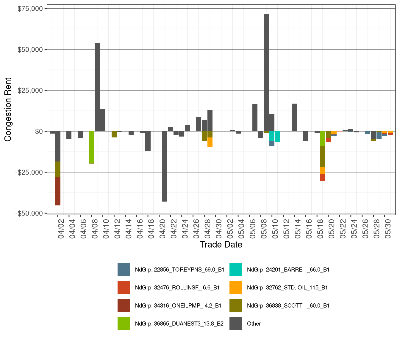
Congestion Rents on Nodal Group Constraints

Figure 4.4 illustrates IFM congestion rents by nodal group constraints. The hourly congestion rent is calculated as the shadow price ($/MWh) of the constraint multiplied by the flow limit (MW). The daily congestion rent is the sum of the hourly congestion rents collected on the constraint for all hours of the trading day.

Figure 4.4: IFM (Day-Ahead) Daily Congestion Rents by Nodal Group Constraints